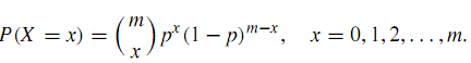
Binomial distribution
The binomial distribution is a discrete probability distribution. It describes the outcome of m independent trials in an experiment. Each trial is assumed to have only two outcomes, either success or failure. If the probability of a successful trial is p, then the probability of having x successful outcomes in an experiment of n independent trials is as follows,
The binomial distribution describes the behavior of a count variable X if the following conditions apply:
1. The number of observations n is fixed.
2. Each observation is independent.
3. Each observation represents one of two outcomes (“success” or “failure”).
4. The probability of “success” p is the same for each outcome.
#R syntax for estimating the probability
dbinom(x, size, prob)
#Example 1:
#Compute the probability of getting five heads in seven tosses of a fair coin.
dbinom(x = 5, size = 7, prob = 0.5)
#Example 2:
#Compute the probability of getting less than or equal four heads in seven tosses of a fair coin.
#Method 1 – Estimate individual probability and sum it together
dbinom(x =0, size = 7, prob = 0.5)
dbinom(x =1, size = 7, prob = 0.5)
dbinom(x =2, size = 7, prob = 0.5)
dbinom(x =3, size = 7, prob = 0.5)
dbinom(x =4, size = 7, prob = 0.5)
#Method 2 – Esimate cumulative probability using inbuilt R function
pbinom(4, 7, 0.5)
#Example 3:
#Suppose there are twelve multiple choice questions in an English class quiz. Each question has five possible answers, and only one of them is correct. Find the probability of having four or less correct answers if a student attempts to answer every question at random
pbinom(4, 12, 0.2)
◙ The expected value (or mean) of a binomial random variable is mp
◙ The variance of a biomial distribution is mp(1 − p)
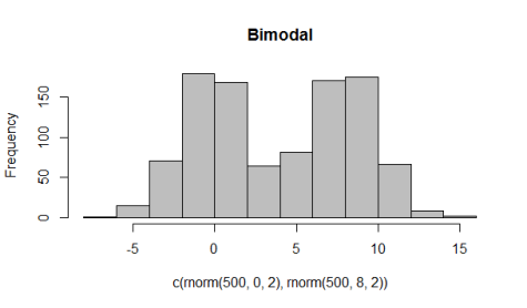
#Visualizing the binomial distribution using histogram plot
hist(c(rnorm(500,0,2),rnorm(500,8,2)),col=”grey”,main=”Bimodal”, breaks = 15)
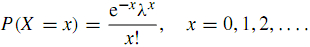
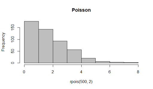
Poisson distribution
The Poisson distribution is the probability distribution of independent event occurrences in an interval. If λ is the mean occurrence per interval, then the probability of having x occurrences within a given interval is:
◙ The mean and variance of a Poisson random variable are both equal to λ.
#R syntax of estimating the probability of Poisson distribution
dpois(x, lambda)
#Example 1:
#According to the Poisson model, the probability of three arrivals at anautomatic bank teller in the next minute, where the average number of arrivals per minute is 0.6, is
dpois(x = 3, lambda = 0.5)
#Cumulative probability is estimated using
ppois()
#We can generate Poisson randomnumbers using the
rpois(n, lambda)
#Example 2:
#Suppose traffic accidents occur at an intersection with a mean rate of 3 per year. Simulate the annual number of accidents for a 12-year period,assuming a Poisson model.
rpois(12, 3)
#Example 3:
#If there are eleven cars crossing a bridge per minute on average, find the probability of having sixteen or more cars crossing the bridge in a particular minute.
ppois(16,11)
#Visualizing the poisson distribution using histrogram plot
hist(rpois(500,2),col=”grey”,main=”Poisson”)
Exponential distribution
The exponential distribution describes the arrival time of a randomly recurring independent event sequence. If μ is the mean waiting time for the next event recurrence, its probability density function is
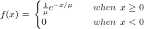
Where mean is reciprocal of the rate parameter.
#R syntax for estimating the probability of exponential distribution
pexp(q, rate)
#Example 1:
#Suppose the service time at a bank teller can be modeled as an exponential random variable with a rate of 3 per minute. Then the probability of acustomer being served in less than 1 minute is
pexp(1, rate = 3)
#The R function can be used to generate n random exponentialvariates.
rexp(n, rate)
#Example 2:
#A bank has a single teller who is facing a queue of 8 customers. The time for each customer to be served is exponentially distributed with rate 2 per minute. We can simulate the service times (inminutes) for the 8 customers.
servicetimes <- rexp(8, rate = 2)
Normal random distribution
A normal random variable X has a probability density function given by
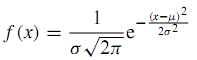
where µ is the expected value of X, and σ2 denotes the variance of X .
◙ The standard normal random variable has mean µ = 0 and standard deviationσ = 1.
◙ The normal density function can be evaluated using the dnorm()
◙ The distribution function can be evaluated using pnorm()
◙ Normal pseudorandom variables can be generated using the rnorm()
#Example 1:
#Assume that the test scores of a college entrance exam fits a normal distribution. Furthermore, the mean test score is 75, and the standard deviation is 15. What is the percentage of students scoring 80 or more in the exam?
pnorm(80, mean=75, sd=15, lower.tail=FALSE)
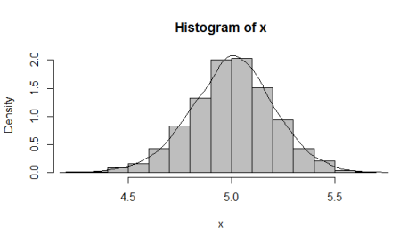
#Visualizing the normal distribution using histrogram plot
x<-rnorm(1000, 5, 0.2)
hist(x,probability = TRUE)
lines(density(x))
Chi-squared Distribution
If X1, X2, …,Xm are m independent random variables having the standard normal distribution, then the following quantity follows a Chi-Squared distribution with m degrees of freedom. Its mean is m, and its variance is 2m.
![]()
#Example 1:
#Find the 97th percentile of the Chi-Squared distribution with 6 degrees of freedom.
qchisq(.97, df=6) # 6 degrees of freedom
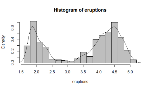
Examining the distribution of a set of data
The distribution can be examined in a number of ways.
# 1 . Generating summary of data
summary(faithful$eruptions)
# 2. Drawing the histogram
hist(eruptions, seq(1.6, 5.2, 0.2), prob=TRUE)
lines(density(eruptions, bw=0.1))