Deep learning basics – part 1

A typical neural network strucutre is shown in below Figure.

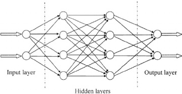
Neural neworks are typically organized in layers. Layers are made up of a number of interconnected nodes which contain an activation function. Each node in a layer is connected in the forward direction to every unit in the next layer. It usually has an input layer, one or more hidden layers and an output layer.

Patterns are presented to the network via the input layer. It communicates to one or more hidden layers where the actual processing is done via a system of weighted connections. The hidden layers then link to an output layer.

✓ Network representation
The equation of a single-layer neural network in matrix form is as follows,
y = Wx
It can be also written in terms of individual components,
y_k = Σ w_kix_i

Where
Input vector x = (x₀,x₁, . . . , x_d)^T
Output vector y = (y₁, . . . , y_k)^T
Weight matrix W:w_ki is the weight from input x_i to output y_k

✓ Weight
A node usually receives many simultaneous inputs, and  each input has its own relative weight. Some inputs are made more important than others. Weight are a measure of an input’s connection strength. These strengths can be modified in response to various training sets and according to a network’s specific topology or its learning rules.

✓ Summation function
The input and weighting coefficients can be combined in many different ways before passing on to the transfer function. The summation function can be sum, max, min, average, or, and. The specific function for combining neural inputs is determined by the chosen network architecture.

✓ Transfer function
The result of the summation function is transformed to a working output through the transfer function. The transfer function can be hyperbolic tangent, linear, sigmoid, sin.

✓ Scaling and limiting
After the transfer function, the result can pass through scale and limit. This scaling simply multiplies a scale factor times the transfer value and then adds an offset. Limiting insures that the scaled result does not exceed an upper, or lower bound.

✓ Output function
Normally, the output is directly equivalent to the transfer function’s result. Some network topologies modify the transfer result to incorporate competition among neighboring processing elements.

✓ Error function/ Backpropagation
The values from the output layer are compared with the expected values and an error is computed for each output unit. The weights connected to the output units are adjusted to reduce those errors. The error estimates of the output units are then used to derive error estimates for the units in the hidden layers. The weight are adjusted to reduce the errors. Finally, the errors are propagated back to the connections stemming from the input units.

✓ Learning function
The purpose of learning funcation is to modify the weights on the inputs of each processing element according to some neural based algorithm.

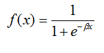
✓ Sigmoid transfer/ activation function
The transfer function for neural networks must be differential as derivative of the transfer function is required for computation of local gradient. Sigmoid is one of the most common forms of transfer function which is used in construction of artificial neural network. It’s represented by following equation,

✓ There are different types of artificial neural networks,
(1) Single layer feed forward network
(2) Multilayer feed forward network
(3) Recurrent network
(4) ….. etc

Neural networks can be trained using supervised and unsupervised manner.

✓ Supervised training – In supervised training, both the inputs and the outputs are provided and the network processes the inputs and compares resulting outputs against the expected outputs. Errors are then propagated back through the system, causing the system to adjust the weights.

✓ Unsupervised training – In this type, the network is provided with inputs but not with desired outputs.

✓ Learning rates
The learning rate depends upon several controllable factors. A slower rate means more time to spend in producing an adequately trained system. In faster learning rates, the network may not be able to make the fine discriminations that are possible with a system learning slowly. Learning rate is positive and it is between 0 and 1.

✓ Learning laws
✶ Hebb’s rule – If a neuron receives an input from another neuron and if both are highly active (same sign), the weight between the two neurons should be strengthened.
✶ Hopfield law – If the desired output and the input are both active or both inactive,
increment the connection weight by the learning rate, otherwise decrement the weight by the learning rate.
✶ The delta rule – This rule is based on the simple idea of continuously modifying the strengths of the input connections to reduce the difference between the desired output value and the actual output of a processing element.
✶ The Gradient Descent rule – This is similar to delta Rule. The derivative of the transfer function is still used to modify the delta error before it is applied to the connection weights. However, an additional proportional constant tied to the learning rate is appended to the final modifying factor acting upon the weight.
✶ Kohonen’s law – The processing elements compete for the opportunity to learn or update their weights. The element with largest output is declared the winner and has the capability of inhibiting its competitors as well as exciting its neighbors. Only the winner is permitted an output and only the winner plus its neighbors are allowed to adjust their connection weights.

✓ Backpropagation for feed forward networks
The backpropagation algorithm is the most commonly used training method for feed forward networks. The main objective in neural network is to find an optimal set of weight parameters, w. The parameters are trained through the training process.

✶ Consider a multi-layer perceptron with k hidden layers. Layer 0 is input layer and layer k+1 is output layer
✶ The weight of j^th unit in layer m and the i^th unit in layer m+1 is denoted by w_ij^m
✶ The input data for a feedforward network training is u(n) =(x₁⁰(n)… x_k⁰(n))
✶ The output is d(n) =(d₁^k+1(n)… d_L ^k+1(n))
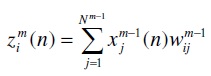
✶ The activation of non-input units is x_i^m+1(n) = f(w_ij^m x_j(n))
✶ A network response obtained in the output layer is y(n) =  (x₁^k+1(n),…, x_L^k+1(n))

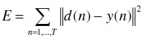
The difference between desired output and neural network output is known as error and it’s quantified as follows,

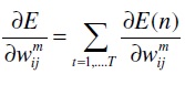
The weights, w, are estimated by minimizing above objective function. This is done by incrementally changing the weights along the direction of the error gradient with respect to weights.

The new weight is

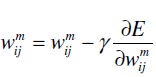
where γ is learning rate. weights are initialized with random numbers. In batch learning mode, new weights are computed after presenting all training samples. One such pass through all samples is called an epoch.

The procedure for one epoch of batch processing is given below.
✶ For each sample n, compute activations of internal and output units (forward pass).

✶  The error propagation term is estimated backward through m = k+1, k, …, 1, for each unit. The error propagation term for output layer is,

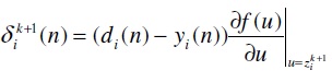
The error propagatin term of hidden layer is estimated using output layer error propagation as bellow,

where, the internal state of unit x_i^m is

✶ Update the weight parameters as bellow,

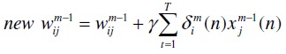
After every such epoch, the error is computed and stop updating the weight when the error falls below a predetermined threshold.